Introduction

I'll be going through a hypothetical scenario at an event ticketing company and describe the data modeling and transformation process in the STAR format. The github repository of the project is linked below.
(https://github.com/Aditya-Tiwari-07/dbt_project)

To setup AWS Redshift, Dbt Cloud and Github for the project please refer the dbt documentation.

To load the Tickit data in AWS Redshift, refer the following guide. (https://docs.aws.amazon.com/redshift/latest/gsg/rs-gsg-create-sample-db.html)

Alternatively, you can also consider setting up the project locally using Dbt core and Duck DB.

Do go through the Tickit DB documentation at the following link to get a feel of the Tickit data warehouse model, so as to better understand the following sections. (https://docs.aws.amazon.com/redshift/latest/dg/c_sampledb.html)

Situation

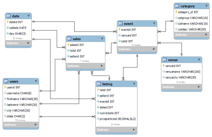
The team handling sales and marketing in the 'Tickit Events' company wants to analyse ticket sales metrics with respect to category, venue, event and more in order to decide the best discounts and promotions strategy. They have a well normalized data warehouse in AWS Redshift, serving as a single source of truth, but its too complex and non-intuitive for the team's data analysts and also slows down their queries due to the large number and complex nature of joins required. The ER diagram for the physical data model of the warehouse is shown below.

They therefore request the data engineering team to create a data mart having an intuitive data model with shortened query times.

Task

As part of the data engineering team, my task is to create the target data model for the data mart and perform the appropriate data transformations on the warehouse data to create a dimensional data model for the data mart, optimized for analytical queries targeting sales metrics.

Action

I strongly encourage referring and running the Dbt SQL transformation models in the project's models folder and querying the created views and tables while reading this section.

1. Selecting the business process: Ticket sale transactions.

2. Declaring the grain: Sale ID, representing the sale of one or more tickets for a particular event listing, by a seller to a buyer.

3. Identifying the Dimensions: Event, Category, Venue, Date, User

4. Identifying the Facts: Sales

5. Creating the conceptual data model for the data mart. The goal is to have all dimension tables directly accessible through the sales fact table. Accordingly, tables and relationships between them are created.

6. Creating the logical data model for the data mart. Here the columns of the tables are decided. The goal here is to remove all foreign keys from dimension tables and place them in the sales fact table.

7. Creating the physical data model for the data mart. Here, the data types of columns and primary and foreign keys are identified. This helps physically implement the data model in the database.

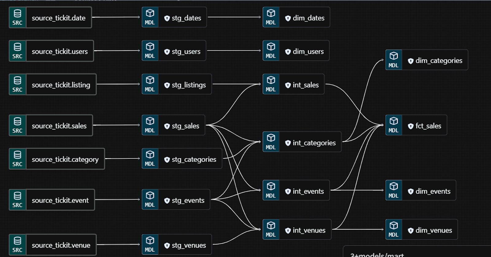
8. Dbt transformations using SQL from source tables to staging layer views. The staging layer mainly serves to rename column names and do basic precalculations. Its important to note that staging views can be used to build multiple intermediate and mart level models. Below is the SQL code for the sales staging view (stg_sales). Note the use of the CTEs to simplify and modularize the code.

9. Dbt transformations using SQL from staging layer views to intermediate layer views. The intermediate layer serves to calculate basic aggregations like MIN, MAX, SUM, COUNT and AVG of sales metrics at the granularity level of the category, event and venue dimensions and to join the Sales and Listing staging views to create a single view. Below is the SQL code for the sales intermediate view, having the facts and foreign keys of both the sales and listing staging views.

10. Dbt transformations using SQL from intermediate and staging layer views to mart layer fact and dimension tables. The mart layer contains the fact and dimension tables tables representing our target data model. This layer materializes the users and date staging views and the categories, venues and events intermediate views into dimension tables. This layer also integrates the foreign keys of the categories, venues and events intermediate views with the sales intermediate view and materializes the result as the sales fact table. The foreign keys in the events intermediate view are not selected to avoid their duplication in the events dimension. This step marks the end of the data transformation process. Below is the SQL code for the sales fact table.

Result

We will now compare the queries and their run times required to fetch a certain set of data from the source layer and the mart layer. Say we want to fetch the top five venues in the 'concerts' category group, based on the number of tickets sold in 2008, ordered in descending order of the number of tickets sold.

Below is the SQL query to fetch this data from the source layer, and its result: -

SELECT v.venueid, v.venuename, SUM(qtysold) AS total_tickets_sold
FROM source_tickit.sales as s
INNER JOIN source_tickit.event as e ON s.eventid = e.eventid
INNER JOIN source_tickit.venue as v ON e.venueid = v.venueid
INNER JOIN source_tickit.category as c ON e.catid = c.catid
INNER JOIN source_tickit.date as d ON s.dateid = d.dateid
WHERE d.year = 2008
    AND c.catgroup='Concerts'
GROUP BY v.venueid, v.venuename
ORDER BY total_tickets_sold DESC
LIMIT 5;

Below is the SQL query to fetch the same data from the mart layer, and its result: -

SELECT v.venue_id, v.venue_name, SUM(qty_sold) AS total_tickets_sold
FROM dbt_atiwari.fct_sales as s
INNER JOIN dbt_atiwari.dim_venues as v ON s.venue_id = v.venue_id
INNER JOIN dbt_atiwari.dim_categories as c ON s.cat_id = c.cat_id
INNER JOIN dbt_atiwari.dim_dates as d ON s.sale_date_id = d.date_id
WHERE d.year = 2008
    AND c.cat_group='Concerts'
GROUP BY v.venue_id, v.venue_name
ORDER BY total_tickets_sold DESC
LIMIT 5;

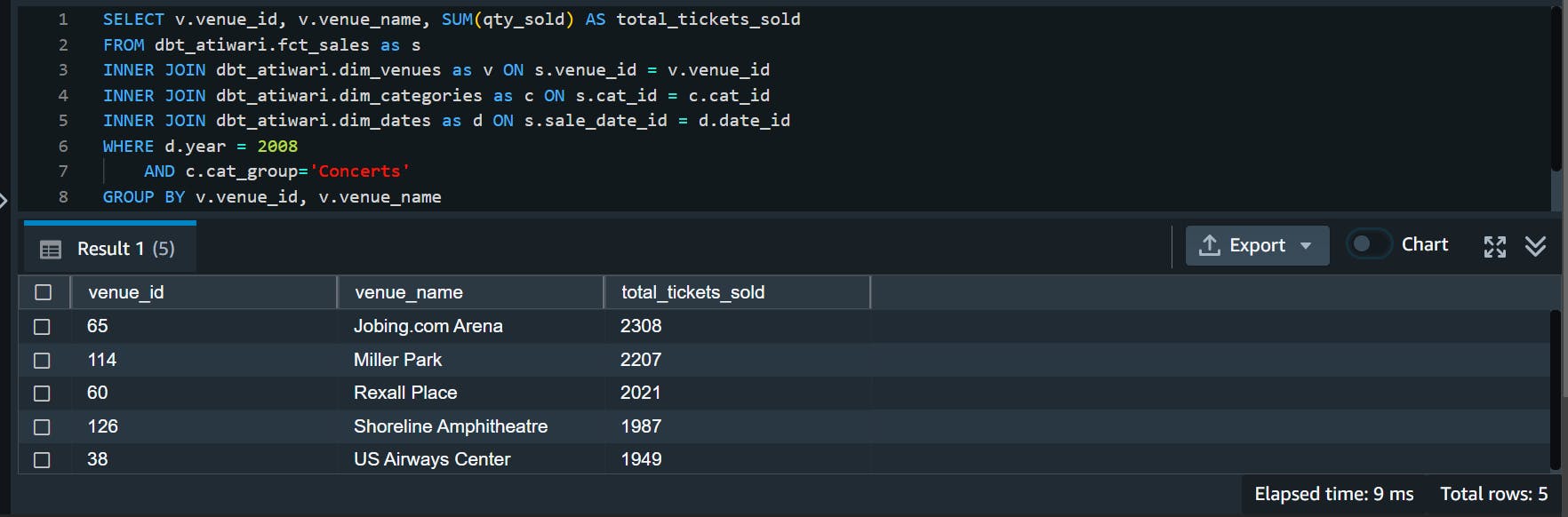
We can see that the query for the mart layer is more intuitive, readable and executes twice as fast, due to less number of SQL joins. This is the main benefit of dimensional modeling and transforming data in warehouses. Intuitive data models, simpler queries and faster execution times increase the productivity of data analysts and data scientists using the data.